Single Model Simulations
Source:vignettes/articles/singleModelSimulations.Rmd
singleModelSimulations.RmdSetting the circuit
This article shows how single model can be simulated using sRACIPE.
suppressWarnings(suppressPackageStartupMessages(library(sRACIPE)))
suppressWarnings(suppressPackageStartupMessages(library(ggplot2)))

racipe <- RacipeSE() # Construct an empty RacipeSE object
data("EMT1") # Load a sample circuit
sracipeCircuit(racipe) <- EMT1
## circuit file successfully loadedracipe## class: RacipeSE
## dim: 16 2000
## metadata(3): annotation nInteractions config
## assays(1): ''
## rownames(16): Zeb1 Snai1 ... Epcam Esrp1
## rowData names(16): Zeb1 Snai1 ... Epcam Esrp1
## colnames: NULL
## colData names(0):Generate a random parameter set
One can initialize the racipe object with experimentally determined parameters or generate a random parameter set and then modify the some or all of the parameters. As we are interested in the trajectories of a single model, we set timeSeries to TRUE.
racipe <- sracipeSimulate(racipe, timeSeries = TRUE, plots = FALSE, genIC = TRUE,
                         genParams = TRUE, integrate = FALSE
                       )
## Generating gene thresholds## generating thresholds for uniform distribution1...
## ====racipe## class: RacipeSE
## dim: 16 1
## metadata(3): annotation nInteractions config
## assays(0):
## rownames(16): Zeb1 Snai1 ... Epcam Esrp1
## rowData names(16): Zeb1 Snai1 ... Epcam Esrp1
## colnames: NULL
## colData names(225): G_Zeb1 G_Snai1 ... Epcam Esrp1Modify the parameters or initial conditions
Notice that the colData changed now and contains the randomly generated parameters and initial conditions. These can be accessed and modified using sracipeParams and sracipeIC accessors.
parameters <- sracipeParams(racipe) # Get the parameters
dim(parameters)
## [1] 1 209parameters["G_Zeb1"]
##     G_Zeb1
## 1 32.35886parameters[,2]
## [1] 10.32762parameters["G_Zeb1"] <- 10*parameters["G_Zeb1"] # modify parameters parameters[,2] <- 50 # modify parameters sracipeParams(racipe) <- parameters # change the parameters to modified values racipe$G_Zeb1
## [1] 323.5886## [1] 16 1ic[1]
## [1] 0.09892328ic[1] <- 10 # modify initial condition sracipeIC(racipe) <- ic # change the ic to modified values
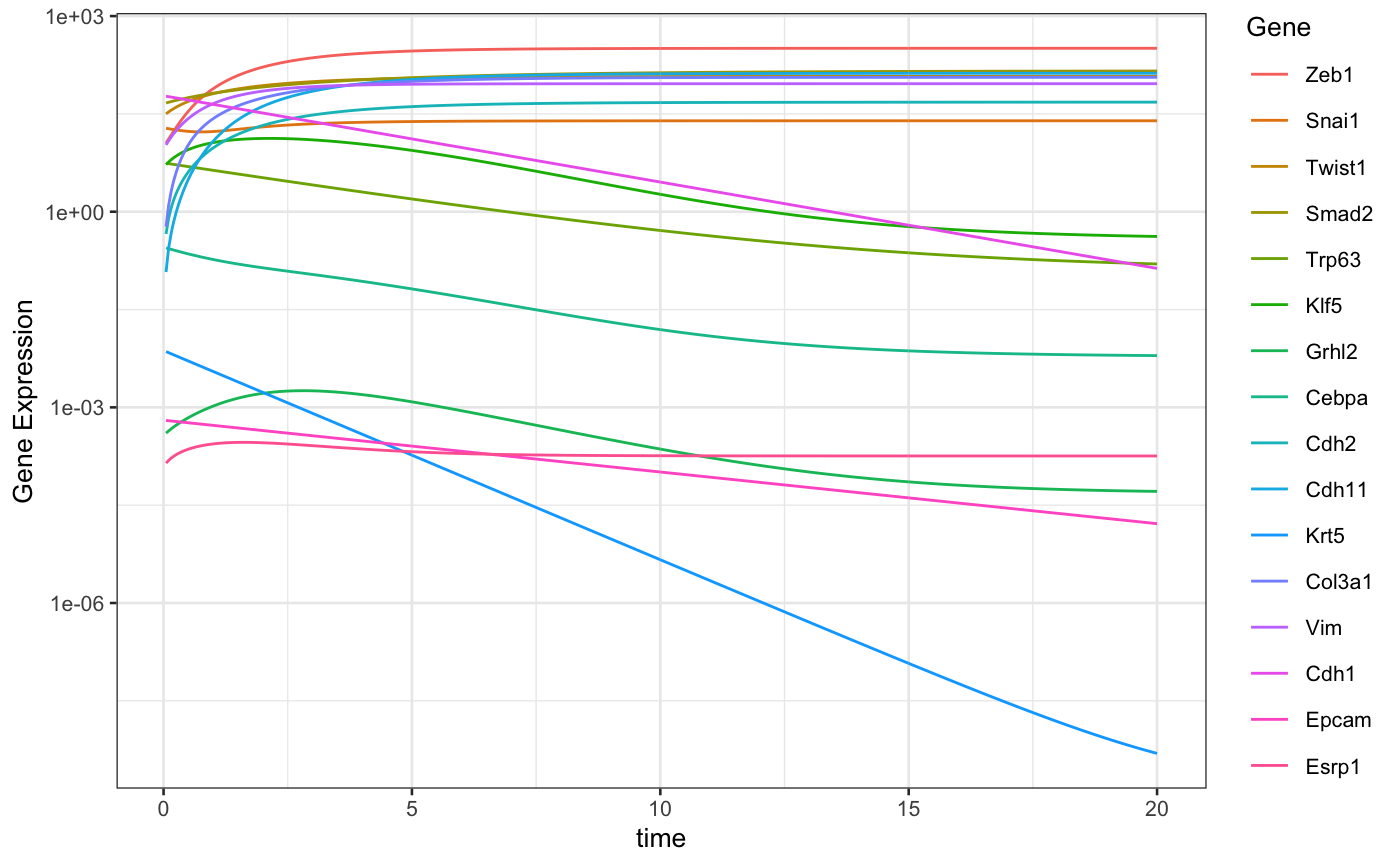
Simulate with modified values
racipe <- sracipeSimulate(racipe, timeSeries = TRUE, plots = FALSE, genIC = FALSE,
                         genParams = FALSE, integrate = TRUE,
                        simulationTime  = 20,
                       integrateStepSize = 0.05
                       )
## ====# Function to plot data sracipePlotTS <- function(plotData, ...){ plotData <- t(plotData) sexprs <- stack(as.data.frame(plotData)) colnames(sexprs) <- c("geneExp", "Gene") sexprs$time <- rep(as.numeric(rownames(plotData)), ncol(plotData)) theme_set(theme_bw(base_size = 10)) ggplot2::qplot(time, geneExp, data = sexprs, group = Gene, colour = Gene, geom = "line", ylab = "Gene Expression", xlab = "time" ) } plotData <- sracipeGetTS(racipe) p <- sracipePlotTS(plotData) p + scale_y_log10() # Use log scale
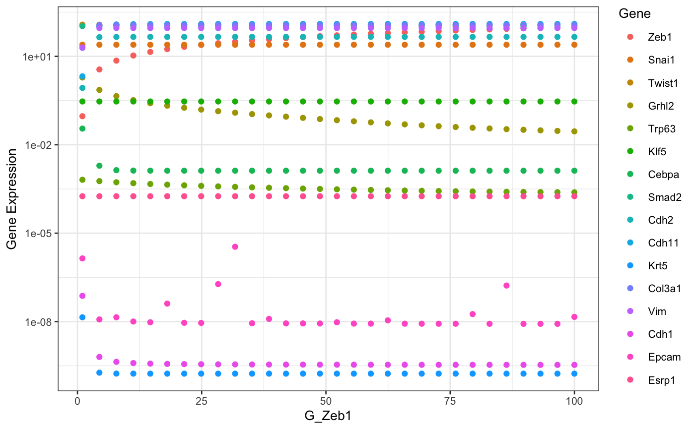
Parameter perturbation
The role of parameter perturbation can be studied by slowly changing one parameter while keeping the other paramters constant. Here we will simulate a large number of models with same parameters except for the parameter being perturbed. We start with a random initial condition each time to capture multiple attractors incase the system is multistable.
selectedParameter <- "G_Zeb1" # parameter to be perturbed
parMin <- 1 # Minimum value of parameter
parMax <- 100 # Maximum value of parameter
nModels <- 30 # Number of models. Parameter value will be uniformly sampled
# nModels times from parMin to parMax.

parameters <- sracipeParams(racipe)
newParameters <- parameters[rep(seq_len(nrow(parameters)), nModels),]
tmpValue <- seq(from = as.numeric(parMin),
                  to = as.numeric(parMax),
                  length.out = nModels)
newParameters[selectedParameter] <- tmpValue

circuit <- sracipeCircuit(racipe)
rs <- sracipeSimulate(circuit, genIC = TRUE, genParams = TRUE, integrate = FALSE,
                          numModels = nModels)
## circuit file successfully loaded## Generating gene thresholds## generating thresholds for uniform distribution1...
## ========================================sracipeParams(rs) <- newParameters # Modify parameters etc rs <- sracipeSimulate(rs, genIC = FALSE, genParams = FALSE, integrate = TRUE, numModels = nModels, simulationTime = 100)
## ========================================# Plot the steady state values library(ggplot2) sexprs <- assay(rs,1) sexprs <- reshape2::melt(t(sexprs)) colnames(sexprs) <- c("bifurParameter","Gene","geneExp") modParameter <- rep(tmpValue,times = dim(rs)[1]) sexprs$modParameter <- modParameter theme_set(theme_bw(base_size = 10)) p <- ggplot2::ggplot(sexprs) + geom_point(aes(x=modParameter,y=geneExp,color = Gene)) + xlab((selectedParameter)) + ylab("Gene Expression") p + scale_y_log10() # Use log scale